Introduction:
With COVID limiting where people can play their instruments on campus, performances and recordings this semester may not sound like they normally would in their typical spaces. As musicians, that’s why we decided to bring the rooms to the player! Through our convolution reverb room simulation, people can make their recordings sound as if they were actually playing in a certain room on campus. To get to our final result, we had to take measurements in each room we wanted to simulate and then analyze the data using MATLAB. We should first explain though, before anything, the concept behind convolution reverb and why we carried out measurements and calculations the way we did.
Background:
Convolution reverb refers to the process of digitally simulating a space. Any room can be emulated if you have the impulse response of that room and an input signal (someone singing or playing an instrument, for example). This is where convolution reverb gets its name, since the calculation to get the end result is called the convolution between the impulse response and the input signal. This is necessary because a room can be thought of as a linear time-invariant (LTI) system, for which a convolution calculation is necessary to carry out.
The input signals we used were dry signals of an oboe and a baritone saxophone, and the impulse response of each room was taken by popping balloons. This is a common method used to get impulse responses of rooms because it is a quick, loud sound that excites all the frequencies of the room without much external interference. That is exactly what an impulse response is: how a space reacts to an external change. Getting the response of frequencies in the room allows us to apply the convolution to an audio signal so that the end result is a signal that has the same response as it would if it were in the room of the impulse response. In other words, the initial signal will sound as if it were being played in that room.
The impulse response was recorded using a binaural microphone known as a “dummy head”. This way we were able to simulate the room in a 3-D scope rather than a mono image. Depending on where we took the impulse recordings in the room in relation to the dummy head, the convoluted signal will sound from the direction of the recorded balloon pop. For example, if the impulse response was taken to the right of the dummy head, the simulation of an input signal would be panned right.
Taking the convolution of a signal and an impulse response, however, is not an easy calculation. There’s a way to simplify the calculation through something called the Fast Fourier Transform (FFT). Convolution in the time domain is equivalent to multiplication in the frequency domain, meaning we can convert our input signal and our impulse response to frequency domain functions and do much easier calculations. The FFT allows us to convert signals from the time domain to the frequency domain, so we can use this to acquire the functions for simplified analysis. To get our output signal back to the time domain, we can take the inverse FFT.
Methods and Analysis:
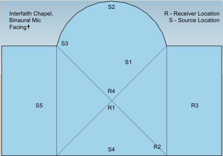
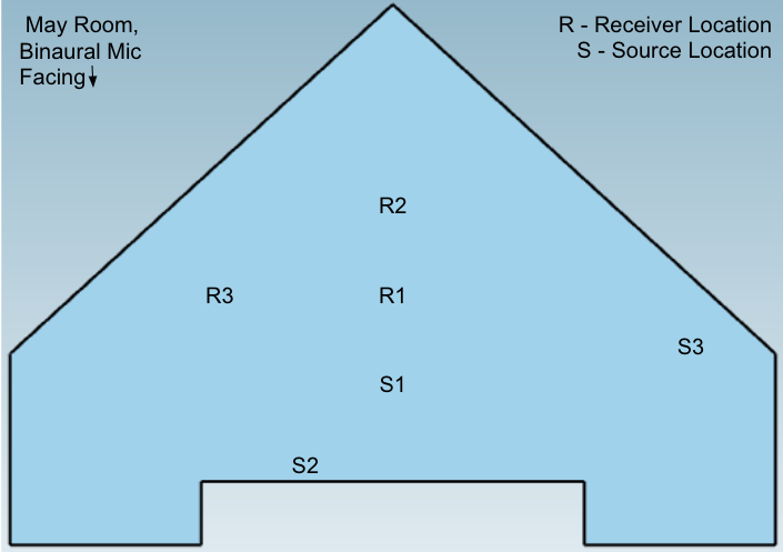
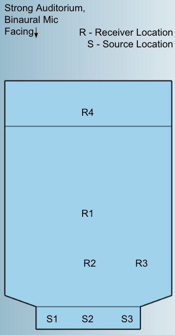
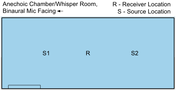
The impulse responses were taken in various rooms on campus, mainly in performance spaces. Responses were also recorded in the anechoic chamber. The recorded impulses were balloon pops, as there are no additional electronic sounds as there would have been if a sine sweep was used. In each room, various source and receiver locations were chosen, with balloons popped at each source location. A binaural microphone was used to record each pop at each receiver position, specifically a Neumann KN100 “dummy head” microphone.
In addition to taking impulse responses at various locations, two performances were recorded in the anechoic chamber, one on oboe and one on a baritone saxophone.
Rough sketches of each space with the source and receiver locations are below.


The input signal and the impulse response are first zero padded to the M + N, where M is the length of the impulse response, and N is the length of the input signal.
The FFT of the padded signal was calculated, and the point by point multiplication was calculated in the frequency domain.
The inverse FFT was taken to bring the signal back to the time domain. The resulting signal is the convolution between these two. It sounds like the dry signal being played in that spot of the room where the impulse response was recorded.
Demos:
While listeners will be able to hear the general reverberation of each space if listening with speakers, listening with headphones will allow for a full binaural experience, where the listener can hear the direction the sound is coming from based on the impulse source and receiver. That is, each recording will sound like the listener is sitting in a specific location in the room, with the performer at the source location. Please note that the recordings from Strong Auditorium do not match the real space as well as other recordings. This is due to curtains being closed for safety purposes on the day that readings were taken.
Conclusions and Future Works:
We were able to successfully recreate the sound of rooms across campus through analysis of the impulse response from each room. The impulse response was captured through recording balloon pops to a binaural microphone known as a “dummy head”. Using a dummy head for recordings gave us a 3-D signal that captured the room sound in a more realistic way than a mono or even stereo source would. Knowing this, we took measurements from different directions (left and right, in front and behind) to capture the full scope of each room. Taking the FFT of the signal in MATLAB to do the convolution between the input signal and the impulse response ultimately gave us our final results. Our next steps would be to use these concepts to create a convolution reverb plug-in, like Altiverb or Space, to work in a DAW in real-time. Even at home, you can now make it sound like you’re playing in a room on the U of R campus!